
California House Price Prediction
With Python and Scikit Learn

Aspiring Data Scientist. I love working with data and creating models from them.
California House Price Prediction Project
In this project I used Python and Scikit Learn Library to predict house prices using the California House Prices dataset from the Scikit learn Library. I used the Linear Regression algorithm to create the model.
In the most simple words, Linear Regression is the supervised Machine Learning model in which the model finds the best fit linear line between the independent and dependent variable i.e it finds the linear relationship between the dependent and independent variable.
Importing the required libraries for the project.
import numpy as np
import pandas as pd

import plotly.express as px
import plotly.graph_objects as go
import plotly.io as pio
pio.templates

import seaborn as sns
import matplotlib.pyplot as plt
%matplotlib inline
Loading the California Housing dataset from the scikit-learn library
from sklearn.datasets import fetch_california_housing
housing = fetch_california_housing()
x = housing.data
y = housing.target

data = pd.DataFrame(x, columns=housing.feature_names) # Using pandas to turn the dataset to a dataframe
data["SalePrice"] = y
data.head() # Getting the first 5 rows of the dataframe
| MedInc | HouseAge | AveRooms | AveBedrms | Population | AveOccup | Latitude | Longitude | SalePrice | |
|---|---|---|---|---|---|---|---|---|---|
| 0 | 8.3252 | 41.0 | 6.984127 | 1.023810 | 322.0 | 2.555556 | 37.88 | -122.23 | 4.526 |
| 1 | 8.3014 | 21.0 | 6.238137 | 0.971880 | 2401.0 | 2.109842 | 37.86 | -122.22 | 3.585 |
| 2 | 7.2574 | 52.0 | 8.288136 | 1.073446 | 496.0 | 2.802260 | 37.85 | -122.24 | 3.521 |
| 3 | 5.6431 | 52.0 | 5.817352 | 1.073059 | 558.0 | 2.547945 | 37.85 | -122.25 | 3.413 |
| 4 | 3.8462 | 52.0 | 6.281853 | 1.081081 | 565.0 | 2.181467 | 37.85 | -122.25 | 3.422 |
Dataset Description
print(housing.DESCR)
.. _california_housing_dataset:

California Housing dataset
--------------------------

**Data Set Characteristics:**

    :Number of Instances: 20640

    :Number of Attributes: 8 numeric, predictive attributes and the target

    :Attribute Information:
        - MedInc        median income in block group
        - HouseAge      median house age in block group
        - AveRooms      average number of rooms per household
        - AveBedrms     average number of bedrooms per household
        - Population    block group population
        - AveOccup      average number of household members
        - Latitude      block group latitude
        - Longitude     block group longitude

    :Missing Attribute Values: None

This dataset was obtained from the StatLib repository.
https://www.dcc.fc.up.pt/~ltorgo/Regression/cal_housing.html

The target variable is the median house value for California districts,
expressed in hundreds of thousands of dollars ($100,000).

This dataset was derived from the 1990 U.S. census, using one row per census
block group. A block group is the smallest geographical unit for which the U.S.
Census Bureau publishes sample data (a block group typically has a population
of 600 to 3,000 people).

An household is a group of people residing within a home. Since the average
number of rooms and bedrooms in this dataset are provided per household, these
columns may take surpinsingly large values for block groups with few households
and many empty houses, such as vacation resorts.

It can be downloaded/loaded using the
:func:`sklearn.datasets.fetch_california_housing` function.

.. topic:: References

    - Pace, R. Kelley and Ronald Barry, Sparse Spatial Autoregressions,
      Statistics and Probability Letters, 33 (1997) 291-297
Getting the number of rows and columns in the dataset
print(data.shape)
(20640, 9)
This tells us that we have 20640 rows and 9 columns in the dataset.
data.info()
Gives us the datatypes and checks if there are missing values in the columns RangeIndex: 20640 entries, 0 to 20639 Data columns (total 9 columns):
 #   Column      Non-Null Count  Dtype
---  ------      --------------  -----
 0   MedInc      20640 non-null  float64
 1   HouseAge    20640 non-null  float64
 2   AveRooms    20640 non-null  float64
 3   AveBedrms   20640 non-null  float64
 4   Population  20640 non-null  float64
 5   AveOccup    20640 non-null  float64
 6   Latitude    20640 non-null  float64
 7   Longitude   20640 non-null  float64
 8   SalePrice   20640 non-null  float64
dtypes: float64(9)
memory usage: 1.4 MB
data.describe()
Gives us the count,mean,standard deviation etc of the dataset
| MedInc | HouseAge | AveRooms | AveBedrms | Population | AveOccup | Latitude | Longitude | SalePrice | |
|---|---|---|---|---|---|---|---|---|---|
| count | 20640.000000 | 20640.000000 | 20640.000000 | 20640.000000 | 20640.000000 | 20640.000000 | 20640.000000 | 20640.000000 | 20640.000000 |
| mean | 3.870671 | 28.639486 | 5.429000 | 1.096675 | 1425.476744 | 3.070655 | 35.631861 | -119.569704 | 2.068558 |
| std | 1.899822 | 12.585558 | 2.474173 | 0.473911 | 1132.462122 | 10.386050 | 2.135952 | 2.003532 | 1.153956 |
| min | 0.499900 | 1.000000 | 0.846154 | 0.333333 | 3.000000 | 0.692308 | 32.540000 | -124.350000 | 0.149990 |
| 25% | 2.563400 | 18.000000 | 4.440716 | 1.006079 | 787.000000 | 2.429741 | 33.930000 | -121.800000 | 1.196000 |
| 50% | 3.534800 | 29.000000 | 5.229129 | 1.048780 | 1166.000000 | 2.818116 | 34.260000 | -118.490000 | 1.797000 |
| 75% | 4.743250 | 37.000000 | 6.052381 | 1.099526 | 1725.000000 | 3.282261 | 37.710000 | -118.010000 | 2.647250 |
| max | 15.000100 | 52.000000 | 141.909091 | 34.066667 | 35682.000000 | 1243.333333 | 41.950000 | -114.310000 | 5.000010 |
Exploratory Data Analysis of the Dataset
Exploratory Data Analysis is a data analytics process to understand the data in depth and learn the different data characteristics, often with visual means. This allows you to get a better feel of your data and find useful patterns in it.
data.isnull().sum()
Gives the sum of null values in the dataset columns. In this case there are none.
MedInc        0
HouseAge      0
AveRooms      0
AveBedrms     0
Population    0
AveOccup      0
Latitude      0
Longitude     0
SalePrice     0
dtype: int64
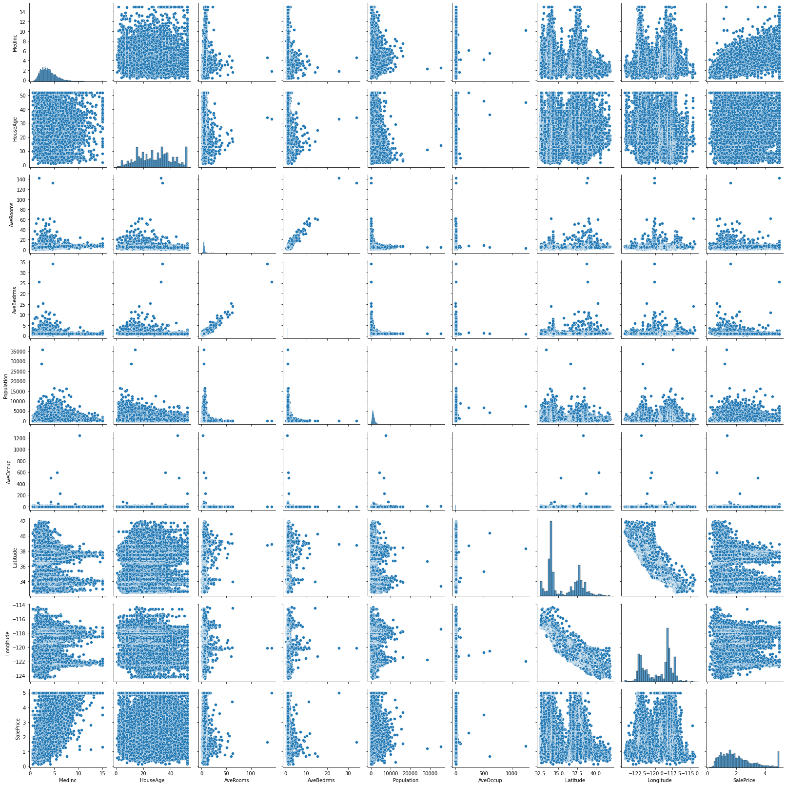
Plot Diagrams
sns.pairplot(data, height=2.5)
plt.tight_layout()
Getting the distribution plot
sns.distplot(data['SalePrice']);
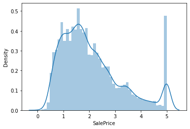
Getting the Skewness and Kurtosis Values
Skewness refers to a distortion or asymmetry that deviates from the symmetrical bell curve, or normal distribution, in a set of data. If the curve is shifted to the left or to the right, it is said to be skewed.
Kurtosis is a measure of the combined weight of a distribution's tails relative to the center of the distribution. When a set of approximately normal data is graphed via a histogram, it shows a bell peak and most data within three standard deviations (plus or minus) of the mean.
print("Skewness: %f" % data['SalePrice'].skew())
print("Kurtosis: %f" % data['SalePrice'].kurt())
Skewness: 0.977763
Kurtosis: 0.327870
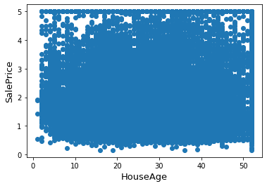
Plotting HouseAge against SalesPrice
fig, ax = plt.subplots()
ax.scatter(x = data['HouseAge'], y = data['SalePrice'])
plt.ylabel('SalePrice', fontsize=13)
plt.xlabel('HouseAge', fontsize=13)
plt.show()
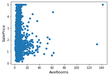
Plotting AveRooms against SalesPrice
fig, ax = plt.subplots()
ax.scatter(x = data['AveRooms'], y = data['SalePrice'])
plt.ylabel('SalePrice', fontsize=13)
plt.xlabel('AveRooms', fontsize=13)
plt.show()
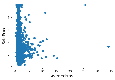
Plotting AveBedrms against SalesPrice
fig, ax = plt.subplots()
ax.scatter(x = data['AveBedrms'], y = data['SalePrice'])
plt.ylabel('SalePrice', fontsize=13)
plt.xlabel('AveBedrms', fontsize=13)
plt.show()
Statistical Calculations
from scipy import stats
from scipy.stats import norm, skew
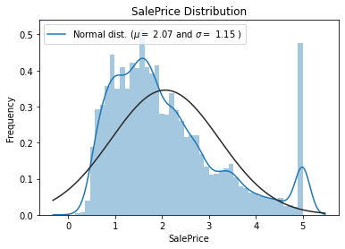
sns.distplot(data['SalePrice'], fit=norm);
(mu, sigma) = norm.fit(data['SalePrice'])
print('\n mu={:.2f} and sigma = {:.2f}\n'.format(mu, sigma))
plt.legend(['Normal dist. ($\mu=$ {:.2f} and $\sigma=$ {:.2f} )'.format(mu, sigma)],
loc='best')
plt.ylabel('Frequency')
plt.title('SalePrice Distribution')
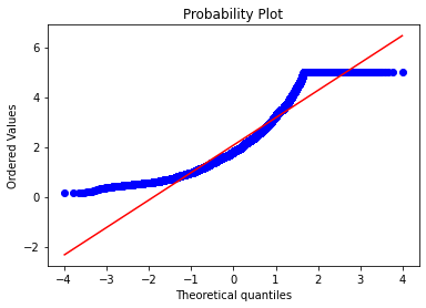
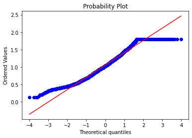
# Get also the QQ-plot
fig = plt.figure()
res=stats.probplot(data['SalePrice'], plot=plt)
plt.show
mu=2.07 and sigma = 1.15
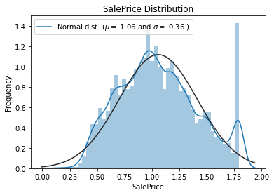
data['SalePrice']=np.log1p(data['SalePrice'])

sns.distplot(data['SalePrice'], fit=norm);

(mu, sigma) = norm.fit(data['SalePrice'])
print('\n mu={:.2f} and sigma = {:.2f}\n'.format(mu, sigma))

plt.legend(['Normal dist. ($\mu=$ {:.2f} and $\sigma=$ {:.2f} )'.format(mu, sigma)],
            loc='best')
plt.ylabel('Frequency')
plt.title('SalePrice Distribution')

fig = plt.figure()
res=stats.probplot(data['SalePrice'], plot=plt)
plt.show
mu=1.06 and sigma = 0.36
Data Correlation
Correlation is a statistical measure that expresses the extent to which two variables are linearly related (meaning they change together at a constant rate). It's a common tool for describing simple relationships without making a statement about cause and effect.
plt.figure(figsize=(10,10))
cor = data.corr()
sns.heatmap(cor, annot=True, cmap=plt.cm.PuBu)
plt.show()
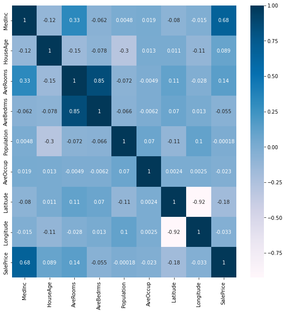
cor_target = abs(cor['SalePrice']) # absolute value of correlation

relevant_features = cor_target[cor_target>0.2] # highly correlated features

names = [index for index, value in relevant_features.iteritems()] # getting the names of the features

names.remove('SalePrice') # removing the target feature

print(names) # printing the features
print(len(names))
['MedInc']
1
Model Building
In this section we build our model which in this case is a Linear Regression Model.
Dividing the data into training and test set
from sklearn.model_selection import train_test_split

x = data.drop('SalePrice', axis=1)
y = data['SalePrice']
x_train, x_test, y_train, y_test = train_test_split(x,y,test_size=0.2, random_state=42)
Number of Rows and Columns of Test and Training Set
print(x_train.shape)
print(x_test.shape)
print(y_train.shape)
print(y_test.shape)
(16512, 8)
(4128, 8)
(16512,)
(4128,)
Importing Linear Regression model from sklearn library
from sklearn.linear_model import LinearRegression

lr = LinearRegression() # Instantiating the Linear Regression Object
lr.fit(x_train, y_train) # Fitting the model
lr.score(x, y)
0.6224456400881904
Getting the Predictions of House Prices
predictions = lr.predict(x_test)

print('Actual value of the house:- $', y_test[0]*100000) # Present Value of the House in dollars
print("Model Predicted Value:-  $", predictions[0]*100000) # Predicted value of the House in dollars
Actual value of the house:- $ 170946.42265012246
Model Predicted Value:-  $ 62758.33553422849
To check the accuracy using Mean Squared Error and Root Mean Squared Error
from sklearn.metrics import mean_squared_error, r2_score

mse = mean_squared_error(y_test, predictions)
rmse=np.sqrt(mse)
print('Mean Squared Error= ', mse)
print('Root Mean Squared Error= ',rmse)

Rsquared=r2_score(y_test, predictions)
print('R^2 Value= ', Rsquared*100,'%')
Mean Squared Error=  0.05034011172872026
Root Mean Squared Error=  0.2243660217785221
R^2 Value=  60.061597228034614 %
GitHub Repository
The GitHub Repository containing the notebook is provided in this link: https://github.com/Nneji123/California-House-Price-Prediction